Analytical shaded relief generated from Digital Elevation Models (DEMs) takes the form of raster image files. Each pixel on the relief image is a grey value calculated from a corresponding elevation on the DEM. This grey value derives from either of two computational methods: vector or difference.
Most applications use the vector method since it allows a finer control over the light direction and is probably more intuitive and easier to use for most cartographers. The vector method uses a physical or empirical law that models how the terrain surface reflects light. A popular model is diffuse reflection.
The difference method uses raster operators applied to a DEM in grid format. Specifically, it involves combining a series of grey tone images derived from the DEM using logical and mathematical operators. This technique is relatively complicated to control and does not yield better results. It is therefore seldom used. For more information, see Böhm’s publications.
Illumination Models
Illumination models can be split in two categories: Local and global models. Local models only consider the interaction between an object and a light source, whereas global models take into account how light interacts between objects, including reflection, transmittance or refraction.
Various authors have produced shaded relief using local models:
| Local Illumination Model | Literature |
| Diffuse reflection | Foley et. al. |
| Phong model | Bui-Tuong |
| Blinn reflection | Blinn |
| Lommel-Seeliger Law | Batson et al. |
| Minnaert’s reflectance function | Minnaert and Horn |
See the literature list for references on publications by these authors.
Global models, such as ray tracing or radiosity are not well suited for cartographic relief shading, since these models are very computation intensive. Local adjustment of illumination yields much more effective cartographic shading than strict adherence to these global illumination models.
Diffuse Reflection
Diffuse reflection assigns each pixel a grey value proportional to the cosine of the angle between the surface normal and the light vector. Diffuse reflection is easy and fast to compute and is therefore widely used for computer graphics.
However, in mountainous areas, comparisons of analytically and manually shaded relief show that the analytical relief often contains undesirable details. By comparison, manual relief accentuates vertical transitions (compare the two figures below) better.
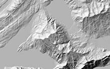
Diffuse reflection and manual shading of Mt. Rigi.
Aspect-Based Shading
The preferred manual style can be simulated in analytical computations by ignoring slope information and basing the shading on aspect only. Various GIS applications sometimes combine aspect-based shading and diffuse reflection. Hereafter an interactive variant is presented.
Aspect-based shading is calculated according to a modified cosine shading equation (Moellering and Kimerling, 1990):
gray value=cos(α)+12
Where α is the angle between aspect and the azimuth of the light direction
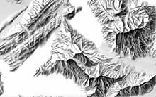
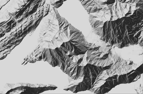
The following figure shows aspect-based shading compared with diffuse illumination.
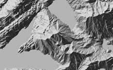
Aspect based shading
Diffuse reflection
Aspect-based shading is well suited for portraying mountainous areas. However, diffuse reflection more accurately depicts flatter and uneven lowlands (compare the upper left corner and the central summit of the two figures above).
The function of the slope of a terrain allows mixing of the two methods of shading. First, a mean or median filter smoothes a matrix containing slope information derived from the DEM. Diffuse reflection and aspect-based shading are then combined as a function of slope according to the following diagram.
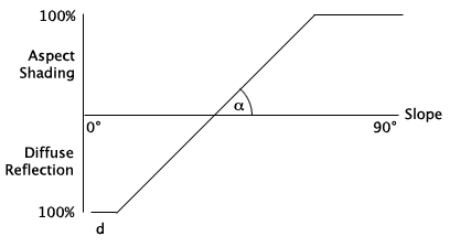
The user of an interactive program combining aspect-based shading and diffuse reflection can adjust the shape of the diagram choosing α and d.
Combination of diffuse reflection and aspect-based shading.